
When you are creating a drop-down list, you will use ‘Data Validation’ to restrict the type of date or values which users enter into cells. To calculate the maximum allowed value in a cell based on a value elsewhere in the workbook, you probably will also use data validation.
If this is your first time to create a drop-down list in Excel, you may not know how Data Validation works and how important it is. Considering making a drop-down list should use the Data Validation feature, it means that Data Validation works importantly. Let’s dive into our post below!
How to Use Data Validation to Create a Drop-Down List in Excel?
Creating a drop-down list in Excel requires you to access ‘Data Validation’ first. You may need to open ‘Data Validation’ after you type the entries you want to appear in the drop-down list and after you choose the cell in the worksheet where you want the drop-down list.
To access ‘Data Validation’, you need to click the ‘Data’ tab in the menu. Then, ‘Data Validation’ can be found under the ‘Data’ menu.

If you cannot click the ‘Data Validation’, the worksheet may be protected or shared. To open Data Validation again, you can try to unlock specific areas of a protected workbook or stop sharing the worksheet. After that, you can try to open ‘Data Validation’ again.
Under ‘Data Validation’, you will find three tabs, including:
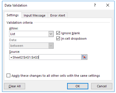
Settings
On the Settings tab, you can click ‘List’ in the Allow box. You need to click in the ‘Source’ box and then choose your list range. For example, in range A2:A9.
Input Message
On the ‘Input Message’ tab, you can tick ‘Show input message when cell is selected’ to show the input message.
Error Alert
On the ‘Error Alert’ tab, you can tick ‘Show error alert after invalid data is entered’. When the users enter the invalid data, you can show this error alert. Make sure to pick an option from the Style box and then type a title and message. Make sure to clear the check box if you do not want a message to show up.
If you are not sure which option to pick in the Style box, you can click ‘Information or Warning’ to show a message which does not stop people from entering data which is not in the drop-down list. The information will show you a message with the ‘i’ icon and Warning will show a message with the ‘!’ icon.
You can then click ‘Stop’ to stop people from entering data which is not in the drop-down list.
Okay, that’s how to use ‘Data Validation’ to create a drop-down list in Excel. Well, using Data Validation is pretty straightforward, isn’t it?
How to Apply Data Validation to Cells?
Data Validation works to restrict the values that you enter into a cell or the type of data that you also enter into a cell. To apply Data Validation to cells, you can do the following steps:
- First, you need to choose the cell you want to create a rule for.
- Then, go to ‘Data’ on the menu and select ‘Data Validation’.
- After Data Validation is open, you need to click the Settings tab.
- Under ‘Allow’ section, you need to choose an option, including:
- Whole Number: This option is used to restrict the cell to accept only whole numbers.
- Decimal: This option is used to restrict the cell to accept only decimal numbers
- List: This option is used to pick data from the drop-down list.
- Date; This option is used to restrict the cell to accept only dates.
- Time: This option is used to restrict the cell to accept only time.
- Text Length: This option is used to restrict the length of the text.
- Custom: This option is used for custom formula
- Under Data, you need to choose a condition.
- Adjust the other required values based on what you selected for Allow and Data.
- Click on the ‘Input message’ tab and make sure to customize a message that you will see when entering data.
- To display the message when you choose or hover over the selected cells, you can choose the ‘Show input message when cell is selected’ checkbox.
- To customize the error message and to select a Style, you need to choose the ‘Error Alert’ tab.
- Last, you can choose OK.
Now, if you try to enter a value which is not valid, an Error Alert will appear with your customized message.
More About Data Valuation in Excel
Under ‘Data Valuation’, you will find two remaining menus including Circle Invalid Data and Clear Validation Circles. Of course, both will have certain functions, regarding the Data Valuation function.
- Circle Invalid Data is used to apply the circles. To do so, you can choose the cells you want to evaluate. Then, go to Data and choose ‘Data Tools’ and click on the ‘Circle Invalid Data’ under Data Valuation.
- Clear Validation Circles is used to quickly remove data validation for a cell. To do so, you can select the cells containing the data you’d like to remove. Then, go to Data and choose ‘Data Tools’ and click on the ‘Clear Validation Circle’ under Data Valuation.
There are so many functions Data Valuation does. For example, if you want to find the cells on the worksheet that have data validation, you can go to the ‘Home’ tab in Excel. In the Editing group, you can click ‘Find & Select’ and then click ‘Data Validation’. Once you’ve found the cells that have data validation, you can then change, copy or remove validation settings.
If you change the validation settings for a cell, it will automatically apply your changes to all other cells that have the same settings. To do so, you can go to the Settings tab and choose to Apply these changes to all other cells with the same settings’ check box.
Additionally, you can also use the ‘Define Name’ command to define a name for the range containing the list. Once creating the list on another worksheet, you can then hide the worksheet containing the list and make sure to protect the workbook, so the users will not have access to the list.

AUTHOR BIO
On my daily job, I am a software engineer, programmer & computer technician. My passion is assembling PC hardware, studying Operating System and all things related to computers technology. I also love to make short films for YouTube as a producer. More at about me…


Leave a Reply